1. 왜 등장했는가
선형 회귀는 연속값을 예측하지만, “생존/사망”처럼 0과 1 사이 확률을 예측해야 할 때 적합하지 않습니다.
선형 회귀의 출력은 음수나 1 초과가 될 수 있어 확률로 해석이 불가능합니다.
Logistic Regression은 시그모이드 함수로 출력을 [0, 1] 범위로 변환해 분류 확률을 제공합니다.
2. 핵심 아이디어 — S자 곡선으로 확률 출력
Logistic Regression은 본질적으로 선형 모델 위에 S자 함수를 씌운 분류기입니다.
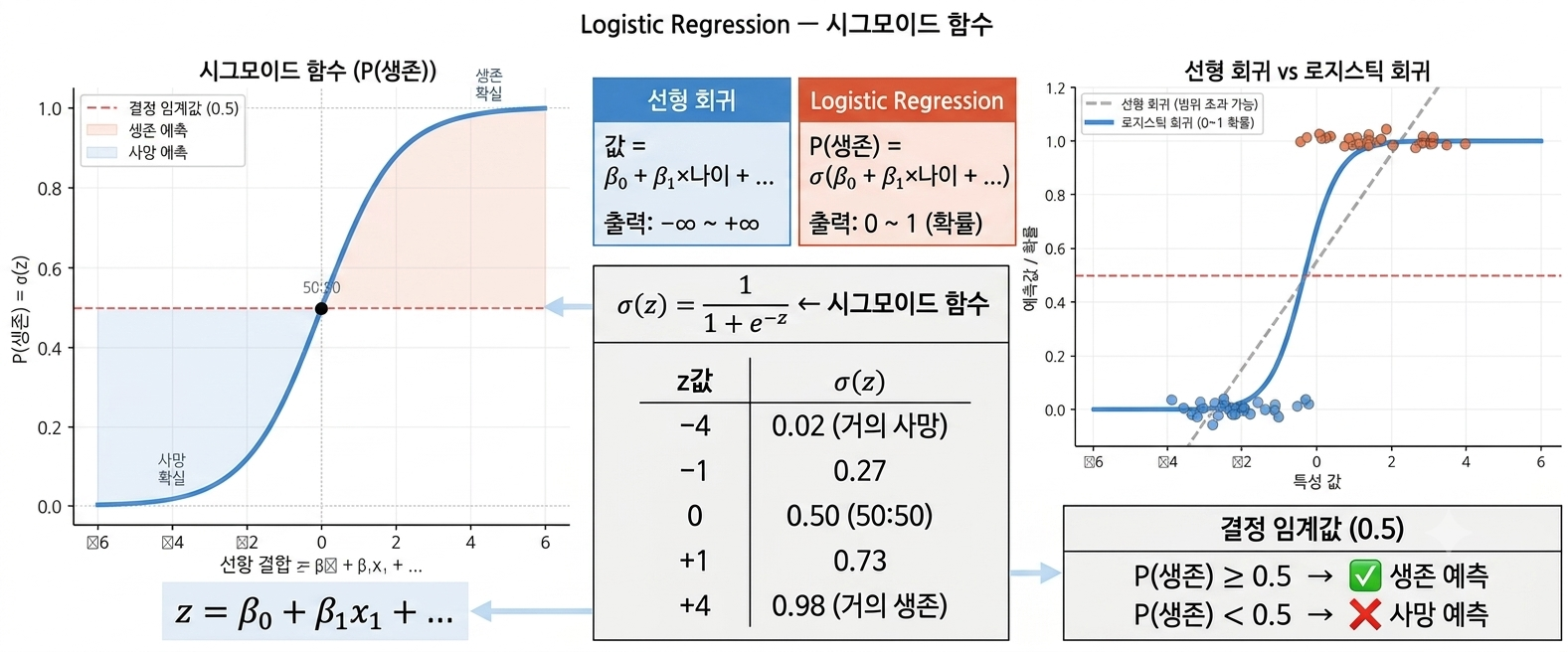
읽는 법 (왼쪽 → 가운데 → 오른쪽 순서로):
① 왼쪽 그래프 — 시그모이드 곡선
x축이 선형 결합 z, y축이 P(생존)입니다.
z값이 아무리 크거나 작아도 σ(z)는 반드시 0과 1 사이에 머뭅니다.
빨간 점선(0.5)을 기준으로 위는 생존, 아래는 사망 예측 영역입니다.
② 가운데 — 선형 회귀 vs Logistic Regression 비교표
선형 회귀는 출력 범위가 -∞~+∞이지만,
로지스틱 회귀는 시그모이드를 씌워 출력이 0~1(확률)로 제한됩니다.
z값 표에서 z=-4면 거의 사망(0.02), z=+4면 거의 생존(0.98)임을 확인하세요.
③ 오른쪽 그래프 — 선형 회귀 vs 로지스틱 회귀 실제 비교
회색 점선(선형 회귀)은 1을 초과하거나 0 미만이 될 수 있지만,
파란 곡선(로지스틱 회귀)은 항상 0~1 범위를 유지합니다.
아래 박스: P(생존) ≥ 0.5이면 생존, < 0.5이면 사망으로 예측합니다. —
3. 실제 예시로 보기 (분류 / 회귀)
예시 1 — 타이타닉 생존 예측 (분류)
1
2
3
4
5
6
7
8
9
10
11
12
13
14
15
16
17
18
19
20
21
| 훈련 데이터:
┌────────┬────────┬─────┬──────────┬──────────┐
│ 이름 │ 성별 │ 나이 │ 객실 등급 │ 생존 여부 │
├────────┼────────┼─────┼──────────┼──────────┤
│ Alice │ 여성 │ 29 │ 1등석 │ ✅ │
│ Bob │ 남성 │ 31 │ 3등석 │ ❌ │
│ Carol │ 여성 │ 45 │ 3등석 │ ✅ │
│ Dave │ 남성 │ 12 │ 2등석 │ ✅ │
│ Eve │ 남성 │ 38 │ 3등석 │ ❌ │
└────────┴────────┴─────┴──────────┴──────────┘
학습된 계수 (예시):
β₀(절편) = -1.2
β₁(성별) = +1.8 (여성일수록 생존 확률 ↑)
β₂(나이) = -0.03 (나이 많을수록 생존 확률 ↓)
β₃(등급) = -0.6 (등급 높을수록 생존 확률 ↓)
새 승객 Frank (남성=0, 나이=25, 3등석):
z = -1.2 + 1.8×0 + (-0.03)×25 + (-0.6)×2
= -1.2 - 0.75 - 1.2 = -3.15
P(생존) = σ(-3.15) ≈ 0.04 → ❌ 사망 예측 (4% 확률)
|
예시 2 — 이메일 응답 시간 예측 (회귀)
1
2
3
4
5
6
7
8
9
10
11
12
13
14
15
16
17
18
19
| 훈련 데이터:
┌──────────────┬──────────┬───────────────┬────────────────────┐
│ 제목 키워드 │ 링크 수 │ 발신자 신뢰도 │ 실제 응답 시간(시) │
├──────────────┼──────────┼───────────────┼────────────────────┤
│ "긴급" 포함 │ 0 │ 0.9 │ 0.5 │
│ 없음 │ 3 │ 0.7 │ 4.2 │
│ "무료" 포함 │ 5 │ 0.2 │ 48.0 │
└──────────────┴──────────┴───────────────┴────────────────────┘
학습된 계수 (선형 회귀):
β₀(절편) = 10.0
β₁("긴급" 포함) = -8.5 (긴급 키워드 있으면 응답 빠름)
β₂(링크 수) = +2.0 (링크 많을수록 응답 느림)
β₃(발신자 신뢰도) = -6.0 (신뢰도 높을수록 응답 빠름)
새 이메일 ("무료" 포함=0, 링크 수=5, 발신자 신뢰도=0.3):
ŷ = 10.0 + (-8.5)×0 + 2.0×5 + (-6.0)×0.3
= 10.0 + 0 + 10.0 - 1.8 = 18.2
예측 응답 시간 ≈ 18.2시간
|
4. 알고리즘 구성 요소
| 구성 요소 | 설명 | 비유 |
|---|
| 선형 결합 z | 특성들의 가중 합산 | 점수 계산 |
| 시그모이드 σ | z를 $0\sim1$확률로 변환 | 점수를 합격 확률로 변환 |
| Log Loss | 예측 확률과 실제 레이블의 차이 | 오답 패널티 |
| 경사 하강법 | 손실을 최소화하는 β 탐색 | 오답률 낮추도록 계수 조정 |
5. 어떻게 계수를 학습하는가
5-1. 손실 함수 (Log Loss / Binary Cross-Entropy)
\[L = -\frac{1}{N}\sum_{i=1}^{N}\left[y_i \log(p_i) + (1-y_i)\log(1-p_i)\right]\]
1
2
| 실제 y=1 (생존), 예측 p=0.9 → L ≈ 0.105 (낮은 손실 ✅)
실제 y=1 (생존), 예측 p=0.1 → L ≈ 2.303 (높은 손실 ❌)
|
5-2. 정규화 (C 파라미터)
\[L_{regularized} = L + \frac{1}{C} \times \|\beta\|\]
1
2
| C 클수록 → 정규화 약함 → 일반 로지스틱 회귀에 가까움 → 과적합 ↑
C 작을수록 → 정규화 강함 → 계수 0에 수렴 → 과소적합 위험
|
6. Logistic Regression 장・단점
6-1. ✅ Logistic Regression 장점
1
2
3
4
5
6
7
8
9
10
11
12
| 1. 확률 출력
→ P(생존)=0.73 같은 확률값 → 의사결정 임계값 조정 가능
2. 계수 해석 가능
→ β > 0: 해당 특성이 클수록 생존 확률 ↑
→ β < 0: 해당 특성이 클수록 생존 확률 ↓
3. 빠른 학습 및 예측
→ 대용량 데이터도 빠름
4. 안정적인 베이스라인
→ 복잡한 모델과 비교하기 위한 기준점
|
6-2. ❌ Logistic Regression이 약한 상황
1
2
3
4
5
6
7
8
| 1. 비선형 패턴
→ 직선 결정 경계 → 복잡한 패턴 포착 불가
2. 특성 간 상호작용
→ 별도로 교호작용 항 수동 추가 필요
3. 이상치
→ 선형 모델 → 이상치에 민감
|
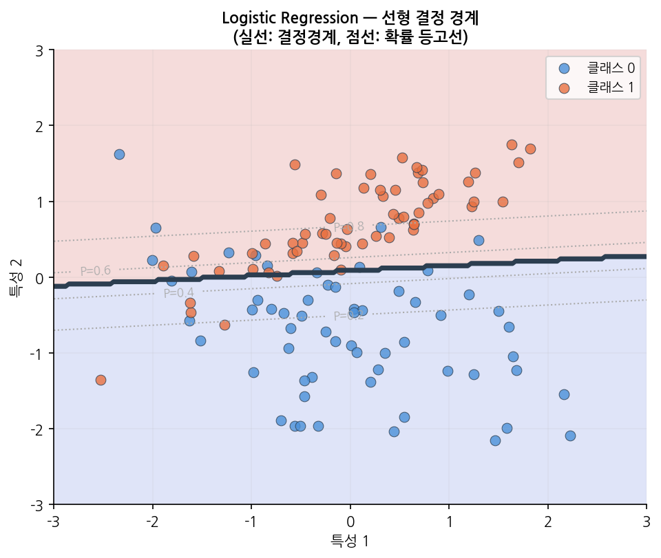
6-2-1. 선형 결정 경계의 한계
Logistic Regression의 가장 큰 약점입니다.
1
2
3
4
5
6
7
8
9
| 로지스틱 회귀 (선형 경계): 트리 기반 (비선형 경계):
나이 나이
│ ○ ○ ● ● ● │ ○ ○ │ ● ● ●
│ ○ ○ ● ● ● │ ○ ○ │ ● ● ●
│○ / ● ● ● │──────┼──────
│ / ○ ● ● │ ○ ● │ ● ●
└────────── 소득 └────────── 소득
직선 하나 직각선 여러 개
|
읽는 법:
진한 선이 결정 경계(P=0.5), 회색 점선이 확률 등고선입니다.
경계에서 멀어질수록 확률이 0 또는 1에 가까워집니다.
이 경계는 항상 직선 하나로 표현됩니다 — 비선형 패턴이 있는 데이터에서는 한계가 있습니다.
해결책 :
1
2
3
4
5
6
7
8
9
10
11
12
13
14
15
16
17
18
| # 방법 1: 다항 특성 추가
from sklearn.preprocessing import PolynomialFeatures
poly = PolynomialFeatures(degree=2)
X_poly = poly.fit_transform(X_train)
# 방법 2: GridSearchCV로 최적 C 탐색
from sklearn.model_selection import GridSearchCV
param_grid = {'C': [0.001, 0.01, 0.1, 1, 10, 100]}
lr_cv = GridSearchCV(
LogisticRegression(penalty='l2', solver='lbfgs', max_iter=1000),
param_grid,
cv=5,
scoring='roc_auc'
)
lr_cv.fit(X_train, y_train)
print(f"Best C : {lr_cv.best_params_['C']}")
print(f"Best AUC : {lr_cv.best_score_:.4f}")
|
7. 한눈에 요약
| 항목 | 내용 |
|---|
| 알고리즘 유형 | 지도학습 / 이진 및 다중 분류 |
| 핵심 아이디어 | 선형 결합 → 시그모이드 → 확률 출력 |
| 결정 경계 | 선형 (직선/평면) |
| 출력 | 클래스 확률 (0~1) |
| 스케일링 필요? | ✅ 필수 (수렴 속도 및 안정성) |
| 핵심 파라미터 | C, penalty, solver |
| 실전 사용 | 빠른 베이스라인, 확률 해석이 중요할 때 |
8. 다른 알고리즘과 무엇이 다른가
Decision Tree vs Logistic Regression
1
2
3
4
5
6
7
| 로지스틱 회귀:
"성별×1.8 + 나이×(-0.03) > 0.5 → 생존"
→ 숫자의 조합. 해석하려면 계수를 읽어야 함.
Decision Tree:
"여성이고, 1등석이면 → 생존"
→ 조건의 나열. 누구나 따라갈 수 있음.
|
| 항목 | Logistic Regression | Decision Tree |
|---|
| 결정 경계 | 선형 | 비선형 (직각) |
| 확률 출력 | ✅ 기본 | ✅ predict_proba |
| 스케일링 | 필수 | 불필요 |
| 해석 | 계수 읽기 | 트리 시각화 |
9. 코드로 보기 — 타이타닉 생존 예측
1
2
3
4
5
6
7
8
9
| from sklearn.linear_model import LogisticRegression
lr = LogisticRegression(
C = 1.0, # 정규화 역수 (클수록 정규화 약함)
penalty = 'l2', # 정규화 방식: 'l1', 'l2', 'elasticnet', None
solver = 'lbfgs', # 최적화 알고리즘
max_iter = 1000, # 수렴 보장을 위해 충분히 크게
random_state = 0
)
|
| Parameter | 설명 | Default |
|---|
C | 정규화 강도의 역수 (클수록 정규화 약함) | 1.0 |
penalty | 정규화 종류 | 'l2' |
solver | 최적화 알고리즘 | 'lbfgs' |
max_iter | 최대 반복 횟수 | 100 |
multi_class | 다중 클래스 처리 방식 | 'auto' |
random_state | 재현성 시드 | None |
C : 정규화 강도 — 가장 중요한 파라미터- 값 변화별 효과
C 클수록 → 정규화 약함 → 훈련 데이터에 더 맞춤 → 과적합 위험C 작을수록 → 정규화 강함 → 가중치 축소 → 과소적합 위험
- 교차 검증으로 최적값 탐색 권장 (보통
[0.001, 0.01, 0.1, 1, 10, 100])penalty : 정규화 방식'l2' → Ridge 정규화 (기본값, 대부분의 solver 지원)'l1' → Lasso 정규화 → solver='liblinear' 또는 'saga' 필요'elasticnet' → solver='saga' 필요None → 정규화 없음
solver : 최적화 알고리즘'lbfgs' → 중소규모, 다중 클래스에 권장 (기본값)'liblinear' → 소규모 데이터, L1 정규화 지원'saga' → 대규모 데이터, L1/ElasticNet 지원
9-1. 전처리
1
2
3
4
5
6
7
8
9
10
11
12
13
14
15
16
17
18
19
20
| import pandas as pd
from sklearn.model_selection import train_test_split
from sklearn.preprocessing import StandardScaler
titanic = pd.read_csv('./Data/Titanic.csv')
titanic['FamSize'] = titanic['SibSp'] + titanic['Parch']
use_cols = ['Survived', 'Pclass', 'Sex', 'Age', 'FamSize', 'Fare', 'Embarked']
titanic = titanic[use_cols].dropna(subset=['Age'])
titanic['Age'] = titanic['Age'].astype(int)
titanic = pd.get_dummies(titanic, columns=['Pclass', 'Sex', 'Embarked'], drop_first=True)
y = titanic['Survived']
X = titanic.drop('Survived', axis=1)
X_train, X_test, y_train, y_test = train_test_split(X, y, test_size=0.25, random_state=0)
# ✅ Logistic Regression은 수렴 속도 개선을 위해 스케일링 권장
scaler = StandardScaler()
X_train = scaler.fit_transform(X_train)
X_test = scaler.transform(X_test)
|
Note: Logistic Regression은 스케일링 없이도 동작하지만, 수렴 속도와 수치 안정성을 위해 StandardScaler를 권장합니다.
9-2. 모델 학습
1
2
3
4
5
6
7
8
9
10
| from sklearn.linear_model import LogisticRegression
lr = LogisticRegression(
C = 1.0, # 정규화 역수 (클수록 정규화 약함)
penalty = 'l2', # 정규화 방식: 'l1', 'l2', 'elasticnet', None
solver = 'lbfgs', # 최적화 알고리즘
max_iter = 1000, # 수렴 보장을 위해 충분히 크게
random_state = 0
)
lr.fit(X_train, y_train)
|
| Parameter | Default | 역할 | 과적합 방향 |
|---|
C | 1.0 | 정규화 역수 | 클수록 과적합 ↑ |
penalty | 'l2' | 정규화 방식 | - |
solver | 'lbfgs' | 최적화 알고리즘 | - |
max_iter | 100 | 최대 반복 수 | - |
C : 가장 중요한 파라미터- 값 변화별 효과
- 클수록 → 정규화 약함 → 과적합 위험 (C=∞가 정규화 없음)
- 작을수록 → 강한 정규화 → 계수가 0에 수렴
- 통상 로그 스케일로 탐색: 0.001, 0.01, 0.1, 1, 10, 100
penalty & solver 조합l2 + lbfgs : 기본값, 소~중규모 데이터l1 + saga : 특성 선택 필요할 때 (Lasso 효과)elasticnet + saga : L1+L2 혼합
max_iter : 수렴 경고 발생 시 늘리기- 기본값 100은 부족할 수 있음 → 1000 권장
9-3. 평가
1
2
3
4
5
6
7
8
9
10
11
12
13
14
15
16
17
18
19
20
| from sklearn.metrics import (
accuracy_score, confusion_matrix,
classification_report, roc_auc_score, RocCurveDisplay
)
import matplotlib.pyplot as plt
pred = lr.predict(X_test)
pred_prob = lr.predict_proba(X_test)[:, 1]
cfx = confusion_matrix(y_test, pred)
sensitivity = cfx[1, 1] / (cfx[1, 0] + cfx[1, 1])
specificity = cfx[0, 0] / (cfx[0, 0] + cfx[0, 1])
roc_auc = roc_auc_score(y_test, pred_prob)
print(f"Accuracy : {accuracy_score(y_test, pred) * 100:.2f}%")
print(f"Sensitivity : {sensitivity * 100:.2f}%")
print(f"Specificity : {specificity * 100:.2f}%")
print(f"ROC AUC : {roc_auc:.4f}")
print()
print(classification_report(y_test, pred, target_names=['Died (0)', 'Survived (1)']))
|
9-4. 계수 해석 — 어떤 특성이 생존에 영향을 주는가
1
2
3
4
5
6
7
8
9
10
11
12
13
14
| import numpy as np
coef = lr.coef_[0]
sorted_idx = np.argsort(coef)
feature_names = X.columns.tolist()
plt.figure(figsize=(7, 5))
colors = ['tomato' if c > 0 else 'steelblue' for c in coef[sorted_idx]]
plt.barh([feature_names[i] for i in sorted_idx], coef[sorted_idx], color=colors)
plt.axvline(0, color='black', linewidth=0.8)
plt.xlabel('Coefficient (양수=생존↑, 음수=사망↑)')
plt.title('Logistic Regression 계수')
plt.tight_layout()
plt.show()
|
9-5. ROC 곡선
1
2
3
4
5
6
7
8
9
10
| fig, ax = plt.subplots(figsize=(6, 5))
RocCurveDisplay.from_predictions(
y_test, pred_prob, ax=ax,
name=f'Logistic Regression (AUC={roc_auc:.3f})'
)
ax.plot([0, 1], [0, 1], 'k--', linewidth=0.8, label='Random')
ax.set_title('ROC Curve — Titanic Survival')
ax.legend()
plt.tight_layout()
plt.show()
|