[Python] ML-LightGBM

개념

---

데이터가 수백만 건에 달하는 빅데이터 시대, 전통적인 Gradient Boost는 너무 느립니다. 이때 혜성처럼 등장하여 Kaggle과 현업을 휩쓴 모델이 바로 LightGBM입니다. 이름처럼 가볍고 빠른 이 모델의 강력함은 어디서 나오는지 분석합니다.

LightGBM은 Microsoft에서 개발한 빠르고 효율적인 Gradient Boosting 프레임워크입니다. 기존 Gradient Boost의 느린 속도 문제를 두 가지 핵심 기술로 해결했습니다.

---

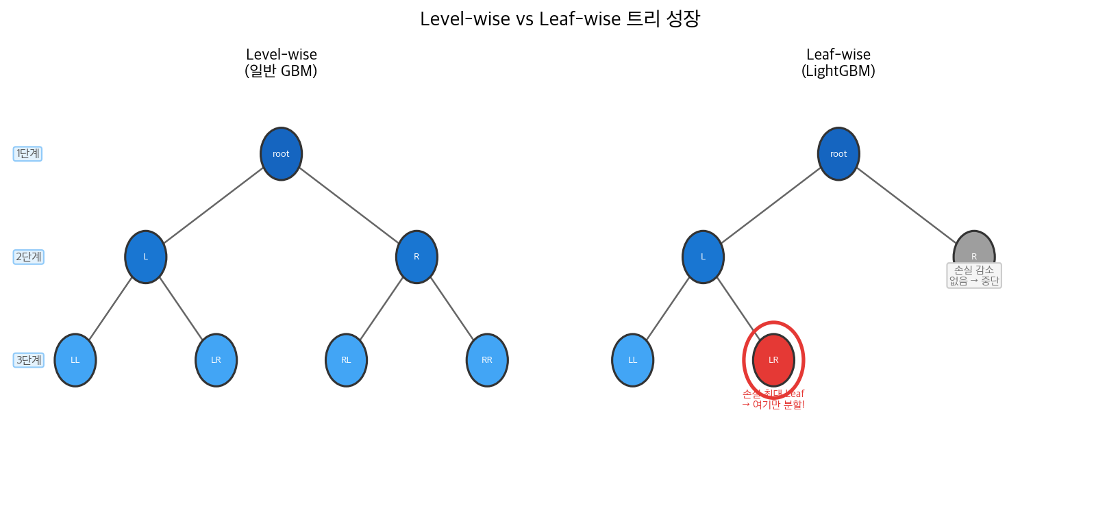
Level-wise(좌)는 같은 깊이의 모든 노드를 분할하지만, Leaf-wise(우)는 손실이 가장 큰 Leaf 하나만 집중 분할합니다.

두 가지 핵심 기술

1. GOSS (Gradient-based One-Side Sampling)

기울기(잔차)가 큰 샘플 → 전부 사용 (학습에 중요)
기울기가 작은 샘플 → 일부만 랜덤 선택

→ 정보 손실 최소화하면서 샘플 수를 줄임
→ 학습 속도 향상

2. EFB (Exclusive Feature Bundling)

동시에 0이 아닌 값을 가지지 않는 희소 변수들을 하나로 묶음

예: 원-핫 인코딩된 변수들은 동시에 1이 되지 않음
→ 여러 변수를 하나로 묶어 변수 수를 효과적으로 줄임
→ 메모리 및 계산 효율 향상

---

Leaf-wise vs Level-wise 트리 성장

Level-wise (일반적인 방식):
같은 깊이의 모든 노드를 분할
→ 균형 잡힌 트리
→ 과적합 위험 낮음

Leaf-wise (LightGBM):
손실 감소가 가장 큰 Leaf 하나만 분할
→ 불균형하지만 정확한 트리
→ 빠른 수렴, 과적합 주의 (max_depth 또는 num_leaves로 제한)

---

언제 사용하는가

사용해야 할 때

상황	이유
대용량 데이터 (수십만 건 이상)	GOSS + EFB로 XGBoost보다 훨씬 빠른 학습
학습 속도가 중요한 실무 환경	동일 성능 기준 가장 빠른 Boosting 계열
범주형 변수가 많을 때	One-Hot Encoding 없이 category 타입으로 직접 처리
메모리가 제한적인 환경	EFB로 변수 수를 효과적으로 압축
캐글 등 경진대회에서 빠른 실험이 필요할 때	빠른 반복 학습으로 하이퍼파라미터 탐색 용이

사용하지 말아야 할 때

상황	이유
소규모 데이터 (수천 건 이하)	Leaf-wise 성장으로 과적합 위험이 높아짐
모델 해석이 핵심인 경우	블랙박스 모델로 개별 예측 설명 어려움
이미지, 텍스트, 시계열	딥러닝 계열이 더 적합

실무 활용 사례

금융: 대규모 신용카드 사기 탐지 (실시간성 + 대용량)
커머스: 수백만 고객의 구매 예측 및 추천
광고: 수억 건 로그 기반 CTR(클릭률) 예측
에너지: 대규모 센서 데이터 기반 설비 이상 탐지

---

핵심 파라미터

파라미터	설명	기본값
n_estimators	트리 수	100
learning_rate	학습률	0.1
num_leaves	트리당 최대 리프 수 (중요)	31
max_depth	최대 깊이 (-1: 제한 없음)	-1
min_child_samples	리프 노드의 최소 샘플 수	20
subsample	샘플 샘플링 비율	1.0
colsample_bytree	변수 샘플링 비율	1.0

num_leaves가 LightGBM의 핵심 파라미터입니다. 2^max_depth보다 작게 설정하는 것이 권장됩니다.

---

실습 — Titanic 생존자 예측

전처리

import pandas as pd
import numpy as np
from sklearn.model_selection import train_test_split

titanic = pd.read_csv('./Data/Titanic.csv')

titanic['FamSize'] = titanic['SibSp'] + titanic['Parch']
use_cols = ['Survived', 'Pclass', 'Sex', 'Age', 'FamSize', 'Fare', 'Embarked']
titanic = titanic[use_cols].dropna(subset=['Age'])
titanic[['Survived', 'Pclass', 'Sex', 'Embarked']] = \
    titanic[['Survived', 'Pclass', 'Sex', 'Embarked']].astype('category')
titanic['Age'] = titanic['Age'].astype('int')
titanic = pd.get_dummies(titanic, columns=['Pclass', 'Sex', 'Embarked'], drop_first=True)

y = titanic['Survived']
X = titanic.drop(['Survived'], axis=1)
X_train, X_test, y_train, y_test = train_test_split(X, y, test_size=0.25, random_state=0)

모델 학습

from lightgbm import LGBMClassifier

LGB = LGBMClassifier(
    n_estimators=200,
    learning_rate=0.05,
    num_leaves=31,
    min_child_samples=20,
    random_state=0,
    verbose=-1
)

LGB.fit(X_train, y_train)

조기 종료 적용

from sklearn.model_selection import train_test_split

X_tr, X_val, y_tr, y_val = train_test_split(X_train, y_train, test_size=0.2, random_state=0)

LGB_ES = LGBMClassifier(
    n_estimators=1000,
    learning_rate=0.05,
    num_leaves=31,
    random_state=0,
    verbose=-1
)

LGB_ES.fit(
    X_tr, y_tr,
    eval_set=[(X_val, y_val)],
    callbacks=[lgb.early_stopping(stopping_rounds=50, verbose=False)]
)

print(f"최적 트리 수: {LGB_ES.best_iteration_}")

범주형 변수 직접 처리

LightGBM의 강점 중 하나입니다. One-Hot Encoding 없이 범주형 변수를 그대로 사용할 수 있습니다.

import pandas as pd
from lightgbm import LGBMClassifier

# One-Hot Encoding 없이 원본 데이터 사용
titanic_cat = pd.read_csv('./Data/Titanic.csv')
titanic_cat['FamSize'] = titanic_cat['SibSp'] + titanic_cat['Parch']
use_cols = ['Survived', 'Pclass', 'Sex', 'Age', 'FamSize', 'Fare', 'Embarked']
titanic_cat = titanic_cat[use_cols].dropna(subset=['Age'])
titanic_cat['Age'] = titanic_cat['Age'].astype('int')

# 범주형 변수를 category 타입으로만 지정
cat_features = ['Pclass', 'Sex', 'Embarked']
for col in cat_features:
    titanic_cat[col] = titanic_cat[col].astype('category')

y_cat = titanic_cat['Survived']
X_cat = titanic_cat.drop('Survived', axis=1)
X_tr_cat, X_te_cat, y_tr_cat, y_te_cat = train_test_split(X_cat, y_cat, test_size=0.25, random_state=0)

LGB_cat = LGBMClassifier(n_estimators=200, random_state=0, verbose=-1)
LGB_cat.fit(X_tr_cat, y_tr_cat,
            categorical_feature=cat_features)  # 범주형 변수 지정

print(f"정확도 : {LGB_cat.score(X_te_cat, y_te_cat) * 100:.2f}%")
# One-Hot Encoding 결과와 성능 비교 가능

성능 평가

from sklearn.metrics import accuracy_score, confusion_matrix

pred = LGB.predict(X_test)
cfx  = confusion_matrix(y_test, pred)

sensitivity = cfx[1, 1] / (cfx[1, 0] + cfx[1, 1])
specificity = cfx[0, 0] / (cfx[0, 0] + cfx[0, 1])

print(f"정확도 : {accuracy_score(y_test, pred) * 100:.2f}%")
print(f"민감도 : {sensitivity * 100:.2f}%")
print(f"특이도 : {specificity * 100:.2f}%")

정확도 : 83.80%
민감도 : 75.00%
특이도 : 89.32%

---

장단점

장점

• XGBoost보다 빠른 학습 속도
• 메모리 효율이 높음
• 범주형 변수 자동 처리 지원
• 대용량 데이터에 적합

단점

• 소규모 데이터에서 Leaf-wise 성장으로 과적합 위험
• num_leaves 등 LightGBM 고유 파라미터 이해 필요
• XGBoost보다 직관적 이해가 어려움

---