| Feature | Type | Description |
|---|
| InvoiceNo | object | 송장번호 |
| StockCode | object | 각 상품(아이템)별로 부여된 5자리 정수번호 |
| Description | object | 상품명 |
| Quantity | int64 | 각 상품의 수량 |
| InvoiceDate | datetime64 | 거래가 발생한 날짜 및 시간 (2010-12-01 ~ 2011-12-09) |
| UnitPrice | float64 | 단위당 상품 가격(영국 파운드 기준) |
| CustomerID | float64 | 각 고객에게 부여된 5자리 정수번호 |
| Country | category | 해당 거래 고객이 거주하는 나라 이름 |
- 분석 내용
- Cohort 분석을 통해 고객 유지율(Customer Retenntion)을 분석하고 시각화
- Cohort Analysis : 시간 흐름에 따라 고객 집단(Cohort)의 행동 변화나 잔존율(Retention)을 추적・분석하는 기법
- 고객이 언제 유입되었는지 기준으로 그룹화하여 시간이 지남에 따라 얼마나 오랬동안 활성화 상태를 유지하는지 파악하는 것을 목표
# Libraries
import pandas as pd
import numpy as np

import matplotlib.pyplot as plt
import seaborn as sns
I. Load Data
# Load Data
df = pd.read_excel("./Data/Cohort_1/Online Retail.xlsx")
df.info()
1
2
3
4
5
6
7
8
9
10
11
12
13
14
15
| <class 'pandas.core.frame.DataFrame'>
RangeIndex: 541909 entries, 0 to 541908
Data columns (total 8 columns):
# Column Non-Null Count Dtype
--- ------ -------------- -----
0 InvoiceNo 541909 non-null object
1 StockCode 541909 non-null object
2 Description 540455 non-null object
3 Quantity 541909 non-null int64
4 InvoiceDate 541909 non-null datetime64[ns]
5 UnitPrice 541909 non-null float64
6 CustomerID 406829 non-null float64
7 Country 541909 non-null object
dtypes: datetime64[ns](1), float64(2), int64(1), object(4)
memory usage: 33.1+ MB
|
II. Data Preprocessing
II-I. 고객 ID (CustomerID)가 NaN인 행 제거
df.dropna(subset = ['CustomerID'], axis = 0, inplace = True)
df
| | InvoiceNo | StockCode | Description | Quantity | InvoiceDate | UnitPrice | CustomerID | Country |
|---|
| 0 | 536365 | 85123A | WHITE HANGING HEART T-LIGHT HOLDER | 6 | 2010-12-01 08:26:00 | 2.55 | 17850.0 | United Kingdom |
| 1 | 536365 | 71053 | WHITE METAL LANTERN | 6 | 2010-12-01 08:26:00 | 3.39 | 17850.0 | United Kingdom |
| 2 | 536365 | 84406B | CREAM CUPID HEARTS COAT HANGER | 8 | 2010-12-01 08:26:00 | 2.75 | 17850.0 | United Kingdom |
| 3 | 536365 | 84029G | KNITTED UNION FLAG HOT WATER BOTTLE | 6 | 2010-12-01 08:26:00 | 3.39 | 17850.0 | United Kingdom |
| 4 | 536365 | 84029E | RED WOOLLY HOTTIE WHITE HEART. | 6 | 2010-12-01 08:26:00 | 3.39 | 17850.0 | United Kingdom |
| … | … | … | … | … | … | … | … | … |
| 541904 | 581587 | 22613 | PACK OF 20 SPACEBOY NAPKINS | 12 | 2011-12-09 12:50:00 | 0.85 | 12680.0 | France |
| 541905 | 581587 | 22899 | CHILDREN’S APRON DOLLY GIRL | 6 | 2011-12-09 12:50:00 | 2.10 | 12680.0 | France |
| 541906 | 581587 | 23254 | CHILDRENS CUTLERY DOLLY GIRL | 4 | 2011-12-09 12:50:00 | 4.15 | 12680.0 | France |
| 541907 | 581587 | 23255 | CHILDRENS CUTLERY CIRCUS PARADE | 4 | 2011-12-09 12:50:00 | 4.15 | 12680.0 | France |
| 541908 | 581587 | 22138 | BAKING SET 9 PIECE RETROSPOT | 3 | 2011-12-09 12:50:00 | 4.95 | 12680.0 | France |
406829 rows × 8 columns
- result
- 541909 rows에서 CutomerID가 비어있는 행이 제거되고 406829 rows만 남음
II-II. 구매한 날짜(월) 추출
- 기준이 월이기 때문에 day는 1로 통일한다.
import datetime as dt

# function for Date(year, month, day)
def get_date(x):
    return dt.datetime(x.year, x.month, 1)

df['InvoiceMonth'] = df['InvoiceDate'].apply(get_date)
df
| | InvoiceNo | StockCode | Description | Quantity | InvoiceDate | UnitPrice | CustomerID | Country | InvoiceMonth |
|---|
| 0 | 536365 | 85123A | WHITE HANGING HEART T-LIGHT HOLDER | 6 | 2010-12-01 08:26:00 | 2.55 | 17850.0 | United Kingdom | 2010-12-01 |
| 1 | 536365 | 71053 | WHITE METAL LANTERN | 6 | 2010-12-01 08:26:00 | 3.39 | 17850.0 | United Kingdom | 2010-12-01 |
| 2 | 536365 | 84406B | CREAM CUPID HEARTS COAT HANGER | 8 | 2010-12-01 08:26:00 | 2.75 | 17850.0 | United Kingdom | 2010-12-01 |
| 3 | 536365 | 84029G | KNITTED UNION FLAG HOT WATER BOTTLE | 6 | 2010-12-01 08:26:00 | 3.39 | 17850.0 | United Kingdom | 2010-12-01 |
| 4 | 536365 | 84029E | RED WOOLLY HOTTIE WHITE HEART. | 6 | 2010-12-01 08:26:00 | 3.39 | 17850.0 | United Kingdom | 2010-12-01 |
| … | … | … | … | … | … | … | … | … | … |
| 541904 | 581587 | 22613 | PACK OF 20 SPACEBOY NAPKINS | 12 | 2011-12-09 12:50:00 | 0.85 | 12680.0 | France | 2011-12-01 |
| 541905 | 581587 | 22899 | CHILDREN’S APRON DOLLY GIRL | 6 | 2011-12-09 12:50:00 | 2.10 | 12680.0 | France | 2011-12-01 |
| 541906 | 581587 | 23254 | CHILDRENS CUTLERY DOLLY GIRL | 4 | 2011-12-09 12:50:00 | 4.15 | 12680.0 | France | 2011-12-01 |
| 541907 | 581587 | 23255 | CHILDRENS CUTLERY CIRCUS PARADE | 4 | 2011-12-09 12:50:00 | 4.15 | 12680.0 | France | 2011-12-01 |
| 541908 | 581587 | 22138 | BAKING SET 9 PIECE RETROSPOT | 3 | 2011-12-09 12:50:00 | 4.95 | 12680.0 | France | 2011-12-01 |
406829 rows × 9 columns
II-III. 고객 별 처음 구매한 날짜 추출
- Why? 처음 구매한 월을 추출하여 얼마나 고객이 오랫동안 유지되는지 알아보기 위함
- 고객 ID (CustomerID)별 처음 구매한 날짜를 추가
df['Cohort First Month'] = df.groupby('CustomerID')['InvoiceMonth'].transform('min')
df
| | InvoiceNo | StockCode | Description | Quantity | InvoiceDate | UnitPrice | CustomerID | Country | InvoiceMonth | Cohort First Month |
|---|
| 0 | 536365 | 85123A | WHITE HANGING HEART T-LIGHT HOLDER | 6 | 2010-12-01 08:26:00 | 2.55 | 17850.0 | United Kingdom | 2010-12-01 | 2010-12-01 |
| 1 | 536365 | 71053 | WHITE METAL LANTERN | 6 | 2010-12-01 08:26:00 | 3.39 | 17850.0 | United Kingdom | 2010-12-01 | 2010-12-01 |
| 2 | 536365 | 84406B | CREAM CUPID HEARTS COAT HANGER | 8 | 2010-12-01 08:26:00 | 2.75 | 17850.0 | United Kingdom | 2010-12-01 | 2010-12-01 |
| 3 | 536365 | 84029G | KNITTED UNION FLAG HOT WATER BOTTLE | 6 | 2010-12-01 08:26:00 | 3.39 | 17850.0 | United Kingdom | 2010-12-01 | 2010-12-01 |
| 4 | 536365 | 84029E | RED WOOLLY HOTTIE WHITE HEART. | 6 | 2010-12-01 08:26:00 | 3.39 | 17850.0 | United Kingdom | 2010-12-01 | 2010-12-01 |
| … | … | … | … | … | … | … | … | … | … | … |
| 541904 | 581587 | 22613 | PACK OF 20 SPACEBOY NAPKINS | 12 | 2011-12-09 12:50:00 | 0.85 | 12680.0 | France | 2011-12-01 | 2011-08-01 |
| 541905 | 581587 | 22899 | CHILDREN’S APRON DOLLY GIRL | 6 | 2011-12-09 12:50:00 | 2.10 | 12680.0 | France | 2011-12-01 | 2011-08-01 |
| 541906 | 581587 | 23254 | CHILDRENS CUTLERY DOLLY GIRL | 4 | 2011-12-09 12:50:00 | 4.15 | 12680.0 | France | 2011-12-01 | 2011-08-01 |
| 541907 | 581587 | 23255 | CHILDRENS CUTLERY CIRCUS PARADE | 4 | 2011-12-09 12:50:00 | 4.15 | 12680.0 | France | 2011-12-01 | 2011-08-01 |
| 541908 | 581587 | 22138 | BAKING SET 9 PIECE RETROSPOT | 3 | 2011-12-09 12:50:00 | 4.95 | 12680.0 | France | 2011-12-01 | 2011-08-01 |
406829 rows × 10 columns
II-IV. 고객이 유지된 날짜 변수 생성
- 월 기준으로 생성
- InoviceDate와 Cohort First Month의 차이는 고객이 유지된 날짜이다.
# Function 날짜의 year, month, day 추출
def get_date_elements(df, column):
    year = df[column].dt.year
    month = df[column].dt.month
    day = df[column].dt.day
    return year, month, day

# 적용
Invoice_year, Invoice_month, _ = get_date_elements(df, 'InvoiceMonth')
Cohort_year, Cohort_month, _ = get_date_elements(df, 'Cohort First Month')
# 사람들이 처음 구매 후 활성화된 기간
year_diff = Invoice_year - Cohort_year
month_diff = Invoice_month - Cohort_month
df['Cohort Retention Period'] = year_diff * 12 + month_diff + 1
df.tail()
| | InvoiceNo | StockCode | Description | Quantity | InvoiceDate | UnitPrice | CustomerID | Country | InvoiceMonth | Cohort First Month | Cohort Retention Period |
|---|
| 541904 | 581587 | 22613 | PACK OF 20 SPACEBOY NAPKINS | 12 | 2011-12-09 12:50:00 | 0.85 | 12680.0 | France | 2011-12-01 | 2011-08-01 | 5 |
| 541905 | 581587 | 22899 | CHILDREN’S APRON DOLLY GIRL | 6 | 2011-12-09 12:50:00 | 2.10 | 12680.0 | France | 2011-12-01 | 2011-08-01 | 5 |
| 541906 | 581587 | 23254 | CHILDRENS CUTLERY DOLLY GIRL | 4 | 2011-12-09 12:50:00 | 4.15 | 12680.0 | France | 2011-12-01 | 2011-08-01 | 5 |
| 541907 | 581587 | 23255 | CHILDRENS CUTLERY CIRCUS PARADE | 4 | 2011-12-09 12:50:00 | 4.15 | 12680.0 | France | 2011-12-01 | 2011-08-01 | 5 |
| 541908 | 581587 | 22138 | BAKING SET 9 PIECE RETROSPOT | 3 | 2011-12-09 12:50:00 | 4.95 | 12680.0 | France | 2011-12-01 | 2011-08-01 | 5 |
[!Caution] - Cohort Retention Period에 +1을 하는 이유
- 코호트 분석에서는 “고객이 코호트에 처음 유입된 달을 기준으로 몇 개월이 경과했는가”를 계산합니다.
- 그런데, 고객이 유입된 같은 달에 다시 구매했다면 경과 개월 수는 0개월이 되어버립니다.
- 분석 관점에서는 이 ’0개월차’를 고객 활동의 첫 번째 달(Month 1)로 간주하는 것이 자연스럽습니다.
- 따라서, 0개월차 → 1개월차로 맞추기 위해 Cohort Retention Period에 +1을 더해줍니다.
III. Visualization
# 실제 활동한 고유 고객의 수를 계산
cohort_data = df.groupby(['Cohort First Month', 'Cohort Retention Period'])['CustomerID'].apply(pd.Series.nunique).reset_index()
cohort_data
| | Cohort First Month | Cohort Retention Period | CustomerID |
|---|
| 0 | 2010-12-01 | 1 | 948 |
| 1 | 2010-12-01 | 2 | 362 |
| 2 | 2010-12-01 | 3 | 317 |
| 3 | 2010-12-01 | 4 | 367 |
| 4 | 2010-12-01 | 5 | 341 |
| … | … | … | … |
| 86 | 2011-10-01 | 2 | 93 |
| 87 | 2011-10-01 | 3 | 46 |
| 88 | 2011-11-01 | 1 | 321 |
| 89 | 2011-11-01 | 2 | 43 |
| 90 | 2011-12-01 | 1 | 41 |
91 rows × 3 columns
- Caution
- 실제 활동한 고유 고객의 수를 계산하는 것은 고객 한 명이 해당 기간 동안 10번 구매했더라도, 그 고객은 1명으로만 집계됨
# create a pivot table
cohort_table = cohort_data.pivot(index = 'Cohort First Month', columns = ['Cohort Retention Period'], values = 'CustomerID')
cohort_table
| Cohort Retention Period | 1 | 2 | 3 | 4 | 5 | 6 | 7 | 8 | 9 | 10 | 11 | 12 | 13 |
|---|
| Cohort First Month | | | | | | | | | | | | | |
| 2010-12-01 | 948.0 | 362.0 | 317.0 | 367.0 | 341.0 | 376.0 | 360.0 | 336.0 | 336.0 | 374.0 | 354.0 | 474.0 | 260.0 |
| 2011-01-01 | 421.0 | 101.0 | 119.0 | 102.0 | 138.0 | 126.0 | 110.0 | 108.0 | 131.0 | 146.0 | 155.0 | 63.0 | NaN |
| 2011-02-01 | 380.0 | 94.0 | 73.0 | 106.0 | 102.0 | 94.0 | 97.0 | 107.0 | 98.0 | 119.0 | 35.0 | NaN | NaN |
| 2011-03-01 | 440.0 | 84.0 | 112.0 | 96.0 | 102.0 | 78.0 | 116.0 | 105.0 | 127.0 | 39.0 | NaN | NaN | NaN |
| 2011-04-01 | 299.0 | 68.0 | 66.0 | 63.0 | 62.0 | 71.0 | 69.0 | 78.0 | 25.0 | NaN | NaN | NaN | NaN |
| 2011-05-01 | 279.0 | 66.0 | 48.0 | 48.0 | 60.0 | 68.0 | 74.0 | 29.0 | NaN | NaN | NaN | NaN | NaN |
| 2011-06-01 | 235.0 | 49.0 | 44.0 | 64.0 | 58.0 | 79.0 | 24.0 | NaN | NaN | NaN | NaN | NaN | NaN |
| 2011-07-01 | 191.0 | 40.0 | 39.0 | 44.0 | 52.0 | 22.0 | NaN | NaN | NaN | NaN | NaN | NaN | NaN |
| 2011-08-01 | 167.0 | 42.0 | 42.0 | 42.0 | 23.0 | NaN | NaN | NaN | NaN | NaN | NaN | NaN | NaN |
| 2011-09-01 | 298.0 | 89.0 | 97.0 | 36.0 | NaN | NaN | NaN | NaN | NaN | NaN | NaN | NaN | NaN |
| 2011-10-01 | 352.0 | 93.0 | 46.0 | NaN | NaN | NaN | NaN | NaN | NaN | NaN | NaN | NaN | NaN |
| 2011-11-01 | 321.0 | 43.0 | NaN | NaN | NaN | NaN | NaN | NaN | NaN | NaN | NaN | NaN | NaN |
| 2011-12-01 | 41.0 | NaN | NaN | NaN | NaN | NaN | NaN | NaN | NaN | NaN | NaN | NaN | NaN |
# change index 형태 변경
cohort_table.index = cohort_table.index.strftime("%B %Y")
cohort_table
| Cohort Retention Period | 1 | 2 | 3 | 4 | 5 | 6 | 7 | 8 | 9 | 10 | 11 | 12 | 13 |
|---|
| Cohort First Month | | | | | | | | | | | | | |
| December 2010 | 948.0 | 362.0 | 317.0 | 367.0 | 341.0 | 376.0 | 360.0 | 336.0 | 336.0 | 374.0 | 354.0 | 474.0 | 260.0 |
| January 2011 | 421.0 | 101.0 | 119.0 | 102.0 | 138.0 | 126.0 | 110.0 | 108.0 | 131.0 | 146.0 | 155.0 | 63.0 | NaN |
| February 2011 | 380.0 | 94.0 | 73.0 | 106.0 | 102.0 | 94.0 | 97.0 | 107.0 | 98.0 | 119.0 | 35.0 | NaN | NaN |
| March 2011 | 440.0 | 84.0 | 112.0 | 96.0 | 102.0 | 78.0 | 116.0 | 105.0 | 127.0 | 39.0 | NaN | NaN | NaN |
| April 2011 | 299.0 | 68.0 | 66.0 | 63.0 | 62.0 | 71.0 | 69.0 | 78.0 | 25.0 | NaN | NaN | NaN | NaN |
| May 2011 | 279.0 | 66.0 | 48.0 | 48.0 | 60.0 | 68.0 | 74.0 | 29.0 | NaN | NaN | NaN | NaN | NaN |
| June 2011 | 235.0 | 49.0 | 44.0 | 64.0 | 58.0 | 79.0 | 24.0 | NaN | NaN | NaN | NaN | NaN | NaN |
| July 2011 | 191.0 | 40.0 | 39.0 | 44.0 | 52.0 | 22.0 | NaN | NaN | NaN | NaN | NaN | NaN | NaN |
| August 2011 | 167.0 | 42.0 | 42.0 | 42.0 | 23.0 | NaN | NaN | NaN | NaN | NaN | NaN | NaN | NaN |
| September 2011 | 298.0 | 89.0 | 97.0 | 36.0 | NaN | NaN | NaN | NaN | NaN | NaN | NaN | NaN | NaN |
| October 2011 | 352.0 | 93.0 | 46.0 | NaN | NaN | NaN | NaN | NaN | NaN | NaN | NaN | NaN | NaN |
| November 2011 | 321.0 | 43.0 | NaN | NaN | NaN | NaN | NaN | NaN | NaN | NaN | NaN | NaN | NaN |
| December 2011 | 41.0 | NaN | NaN | NaN | NaN | NaN | NaN | NaN | NaN | NaN | NaN | NaN | NaN |
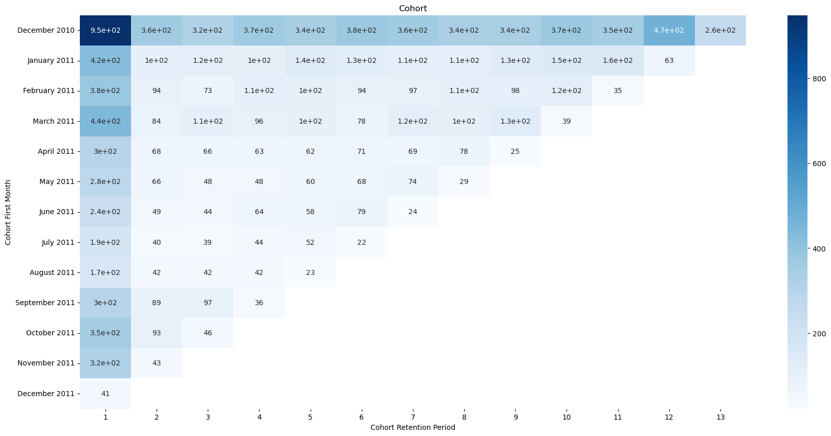
# Visualize our results in heatmap
plt.figure(figsize = (21, 10))
plt.title("Cohort")
sns.heatmap(cohort_table, annot = True, cmap = "Blues")
plt.show()
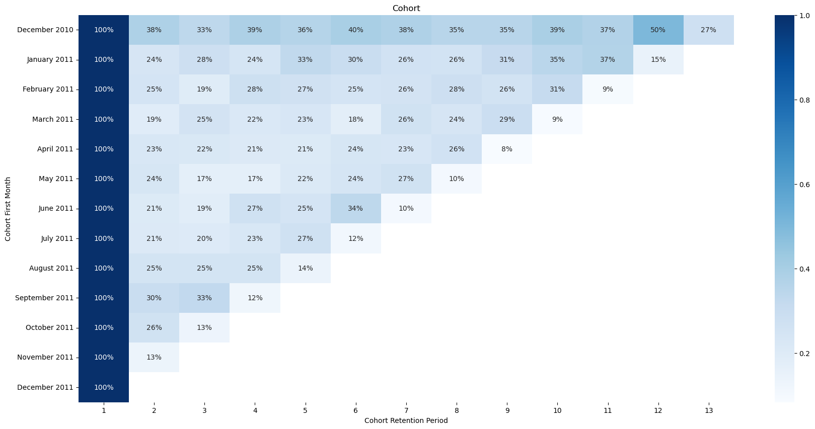
# cohort table for percentage
# 고객 유지율 = 특정 경과 기간의 잔존 고객수 / 코호트 유입 시점의 총 고객 수
new_cohort_table = cohort_table.divide(cohort_table.iloc[:, 0], axis = 0)
new_cohort_table
| Cohort Retention Period | 1 | 2 | 3 | 4 | 5 | 6 | 7 | 8 | 9 | 10 | 11 | 12 | 13 |
|---|
| Cohort First Month | | | | | | | | | | | | | |
| December 2010 | 1.0 | 0.381857 | 0.334388 | 0.387131 | 0.359705 | 0.396624 | 0.379747 | 0.354430 | 0.354430 | 0.394515 | 0.373418 | 0.500000 | 0.274262 |
| January 2011 | 1.0 | 0.239905 | 0.282660 | 0.242280 | 0.327791 | 0.299287 | 0.261283 | 0.256532 | 0.311164 | 0.346793 | 0.368171 | 0.149644 | NaN |
| February 2011 | 1.0 | 0.247368 | 0.192105 | 0.278947 | 0.268421 | 0.247368 | 0.255263 | 0.281579 | 0.257895 | 0.313158 | 0.092105 | NaN | NaN |
| March 2011 | 1.0 | 0.190909 | 0.254545 | 0.218182 | 0.231818 | 0.177273 | 0.263636 | 0.238636 | 0.288636 | 0.088636 | NaN | NaN | NaN |
| April 2011 | 1.0 | 0.227425 | 0.220736 | 0.210702 | 0.207358 | 0.237458 | 0.230769 | 0.260870 | 0.083612 | NaN | NaN | NaN | NaN |
| May 2011 | 1.0 | 0.236559 | 0.172043 | 0.172043 | 0.215054 | 0.243728 | 0.265233 | 0.103943 | NaN | NaN | NaN | NaN | NaN |
| June 2011 | 1.0 | 0.208511 | 0.187234 | 0.272340 | 0.246809 | 0.336170 | 0.102128 | NaN | NaN | NaN | NaN | NaN | NaN |
| July 2011 | 1.0 | 0.209424 | 0.204188 | 0.230366 | 0.272251 | 0.115183 | NaN | NaN | NaN | NaN | NaN | NaN | NaN |
| August 2011 | 1.0 | 0.251497 | 0.251497 | 0.251497 | 0.137725 | NaN | NaN | NaN | NaN | NaN | NaN | NaN | NaN |
| September 2011 | 1.0 | 0.298658 | 0.325503 | 0.120805 | NaN | NaN | NaN | NaN | NaN | NaN | NaN | NaN | NaN |
| October 2011 | 1.0 | 0.264205 | 0.130682 | NaN | NaN | NaN | NaN | NaN | NaN | NaN | NaN | NaN | NaN |
| November 2011 | 1.0 | 0.133956 | NaN | NaN | NaN | NaN | NaN | NaN | NaN | NaN | NaN | NaN | NaN |
| December 2011 | 1.0 | NaN | NaN | NaN | NaN | NaN | NaN | NaN | NaN | NaN | NaN | NaN | NaN |
# create a percentages
plt.figure(figsize = (21, 10))
plt.title("Cohort")
sns.heatmap(new_cohort_table, annot = True, cmap = "Blues", fmt = '.0%')
plt.show()